1.5. Speech Activity Detection (SAD)

Speech Activity Detection enables the computer to differentiate between human speech and absense thereof in a given sound sample. There are several algorithms that allow you to implement SAD. In PySLGR, there are two different approaches to SAD: spectral content analysis and energy based analysis. For an example of spectral based SAD, see example_gmmsad. To further illustrate the functionality of pySLGR’s SAD, we will use the energy based approach in the sections that follow.

1.5.1. Example

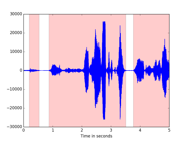
By applying xtalk() to the examples/signals/example.sph file, we can calculate the speech activity in the example signal. We look at the first 5 seconds and notice that the highlighted areas indicate speech activity.

1.5.2. xtalk()

The xtalk() function can be found in the LLFeatures class. The function is used to calculate where speech activity occured. The function itself does not return its calculations but there are several ways to access and use these calculations. They are described in the sections below and include discussions of the following functions:

• apply_sad()
• save_sad_labels()
• save_sad_marks()
• load_sad_labels()
• load_sad_marks()

Note

Marks are only available in MFCCFeatures, not in LLFeatures

1.5.3. apply_sad()

Once calculations have been made using xtalk(), we can remove the non-speech frames from the feature vector. To do so, we use apply_sad(). This does not modify the signal, just the SAD features.

1.5.4. SAD marks and labels

After calculating SAD using xtalk(), the results can be stored in two different ways. We can store them as labels using save_sad_labels(). This function will store the labels in a file of your choosing. The output will be a ‘0’ or ‘1’ indicating whether a frame is not speech or is speech, respectively.

To load labels that have been saved or produced by another program, use load_sad_labels(). Labels can be imported in this manner from any file containing the correct format.

Marks on the other hand can only be stored and loaded from the MFCCFeatures class. Marks work in a similar way to labels, however store the information in a different format. The save_sad_marks() function produces a file in which each line has the following format:

“speech <start_of_speech_activity> <duration_of_speech_activity>”

First is noted the category of activity, which is ‘speech’, then using spaces as delimiters, the starting point of the speech activity is given in seconds followed by the duration of that speech activity (also in seconds).

To load a file of SAD marks, use load_sad_marks().

1.5.5. Putting it all together

To obtain the figure shown in the example, we used xtalk() and save_sad_marks(). The code below shows how to obtain the same image. The code is intended to run from the top level pyslgr directory.

#!/usr/bin/env python

from pyslgr.LLSignal import LLSignal
from pyslgr.MFCCFeatures import MFCCFeatures
import json
import matplotlib.pyplot as plt 
import numpy as np 


sig = LLSignal()
sig.load_sph('example.sph',0)

fp = open('examples/config/lid_config.json', 'r')
c = json.load(fp)
fp.close()

feat_config = c['lid_config']['feat_config']
feat_config['fb_only'] = 'true'

mfcc_config = json.dumps(feat_config)

feats = MFCCFeatures()
feats.process(sig, mfcc_config)
feats.delta(2)
feats.accel(2)

feats.xtalk(0,5,5)

feats.save_sad_marks('example.marks')

marks = []
max_seconds = 5

with open('example.marks') as file:
	lines = file.readlines()
	for line in lines:
		tokens = line.split()
		x = float(tokens[1])
		d = float(tokens[2])
		if(x < max_seconds):
			if (x+d < max_seconds):
				marks.append((x, x+d))
			else:
				marks.append((x, max_seconds))
		else:
			continue

sf = sig.sampling_frequency()
z = range(0, max_seconds*int(sf))
t = (1.0/sf)*np.array(z)
plt.plot(t, sig[0:len(z)])
plt.xlabel('Time in seconds')

for mark in marks:
	plt.axvspan(mark[0], mark[1], facecolor='r', alpha=0.2)

plt.show()